Introduction to Stochastic Variational Inference and Bayesian Neural Networks

---

• The final goal of this notebook is to understand and implement Bayesian Neural Networks (BNNs).
• We must understand the general framework of Bayesian/Probabilistic Machine Learning first.
• This detour will contain more abstractions than BNNs require in the end,
• but it is necessary to describe the general class of optimization problems Pyro is built to tackle
• to properly understand how the bayesian machine learning framework and Pyro are applied to the special case of BNNs.

The notebook therefore starts off by introducing somewhat heavy mathematical machinery,
which we are then going to progressively hide/abstract away with

1. Pyro for arbitrary Bayesian Machine Learning
2. TyXe for Bayesian Neural Networks

Outline

• Introduction
• Outline
• Setup
• Probabilistic Machine Learning
  • Probabilistic Models
  • Bayesian Inference
• Inference in Pyro
  • Stochastic Variational Inference
  • ELBO
  • Pyro Primitives
  • Pyro's "guide" programs
  • Summary
• Example: Variational AutoEncoder
• Example: VAE.model()
• Example: VAE.guide()
• Bayesian Neural Networks
• BNNs in Pyro
• BNNs in TyXe
• References

Setup

Let's make sure we have everything we need.
If you installed the dependencies (including ipykernel) in a virtual/conda environment,
Select Kernel > Change Kernel > environmentname

# run this cell to reset the kernel or select kernel > restart kernel
%reset -s -f 

!jupyter nbextension enable --py widgetsnbextension

Enabling notebook extension jupyter-js-widgets/extension...
      - Validating: OK

import logging
import os

import numpy as np

import matplotlib.pyplot as plt
from matplotlib import rc

import torch
import torch.nn as nn
import torch.utils.data as data
import torchvision

import pyro
import pyro.distributions as dist

assert pyro.__version__.startswith('1.4.0'), f"For TyXe, pyro version must be exactly 1.4.0, not {pyro.__version__}"

# pyro.enable_validation(True)
pyro.distributions.enable_validation(False)
pyro.set_rng_seed(42)

logging.basicConfig(format='%(message)s', level=logging.INFO)

# Set matplotlib settings
%matplotlib inline
plt.style.use('default')

# Is GPU available?
USE_CUDA = torch.cuda.is_available()

USE_CUDA

True

Probabilistic Machine Learning

Most data analysis problems can be understood as elaborations on three basic high-level questions:

1. What do we know about the problem before observing any data? (Priors)
2. What conclusions (inferences) can we draw from data given our prior knowledge? (Posteriors)
3. Do these conclusions make sense? (Uncertainty Quantification)

In the probabilistic or Bayesian approach to data science and machine learning,
we formalize these in terms of mathematical operations on probability distributions.

Probabilistic Models

We express everything we know about the variables in a problem and the relationships between them in the form of a *probabilistic model*:

1. observations ${\bf x}$
2. latent random variables ${\bf z}$
3. parameters $\theta$

It usually has a joint density function of the form

$$p_{\theta}({\bf x}, {\bf z}) = p_{\theta}({\bf x}|{\bf z}) p_{\theta}({\bf z})$$

The distribution over latent variables $p_{\theta}({\bf z})$ in this formula is called the *prior, and the distribution over observed variables given latent variables $p_{\theta}({\bf x}|{\bf z})$ is called the likelihood*.

Probabilistic models are often depicted in a standard graphical notation (Bayesian Networks):

Pyro >= 1.8.0 supports rendering arbitrary functions containing Pyro expressions as graphical models using pyro.render_model(function, model_args=(x,y))

Bayesian Inference, Learning and Evaluation

Once we have specified a model, Bayes' rule tells us how to use it to perform *inference, or draw conclusions about latent variables from data, by computing the posterior distribution* over $\bf z$

$$ p_{\theta}({\bf z} | {\bf x}) = \frac{p_{\theta}({\bf x} , {\bf z})}{ \int \! p_{\theta}({\bf x} , {\bf z})\; d{\bf z} } $$

To check the results of modeling and inference, we would like to know how well a model fits observed data $x$, which we can quantify with the *evidence* (or *marginal likelihood*)

$$p_{\theta}({\bf x}) = \int \! p_{\theta}({\bf x} , {\bf z})\; d{\bf z} $$

and also to make predictions for new data (and sample new data points!), which we can do with the *posterior predictive distribution*

$$p_{\theta}(x' | {\bf x}) = \int \! p_{\theta}(x' | {\bf z}) p_{\theta}({\bf z} | {\bf x})\; d{\bf z} $$

It is often desirable to *learn* the parameters $\theta$ of our models from observed data $x$, which we can do by maximizing the evidence:

$$\theta_{\rm{max}} = \rm{argmax}_\theta p_{\theta}({\bf x}) = \rm{argmax}_\theta \int \! p_{\theta}({\bf x} , {\bf z}) \; d{\bf z} $$

Some Bayesian Inference Algorithms

One naive way to set the parameters $\theta$ is Maximum Likelihood Estimation (MLE):

$$\theta_{\rm{max}} = \rm{argmax}_\theta p_{\theta}({\bf x} | {\bf z})$$

The converse of MLE is to maximize the posterior, this is called Maximum-a-posteriori Estimation (MAP) and requires picking a Prior $p_\theta({\bf z})$:

$$ \theta_{\rm{max}} = \rm{argmax}_\theta p_\theta({\bf z} | {\bf x}) = \rm{argmax}_\theta \frac{p_\theta({\bf x} | {\bf z}) p_\theta({\bf z})}{ \int_Z \! p_\theta({\bf x} | {\bf z})p_\theta({\bf z})\; d{\bf z} } = \rm{argmax}_\theta p_\theta({\bf x} | {\bf z} ) p_\theta({\bf z}) $$

(Wee see that Bayes Theorem implies MLE is actually the most naive case of MAP with the Prior $p_\theta({\bf z})$ being uniform!)

• Non-Bayesian Machine Learning is just MLE.
• Many more Bayesian Inference Algorithms exist, also e.g. Expectation Maximization, see also the List of Pyro's built in Inference Algorithms
• The algorithm we care about is Stochastic variational inference.

Inference in Pyro

Stochastic Variational Inference (SVI)

• Problem: To get any of the quantities above exactly (especially the posterior) requires performing integrals that are impossible or computationally intractable
• Solution: Pyro supports many different approximate inference algorithms; the flagship is stochastic variational inference (SVI)
• SVI is a very general algorithm for finding $\theta_{\rm{max}}$ and computing a tractable approximation $q_{\phi}({\bf z})$ to the true, unknown posterior $p_{\theta_{\rm{max}}}({\bf z} | {\bf x})$
• Mathematicians call $q_{\phi}({\bf z})$ variational distribution or approximate posterior; Pyro calls this guide
• SVI converts the intractable integrals into optimization of a functional of $p_\theta$ and $q_\phi$
• More precise, mathematical discussion & references in Pyro's SVI tutorials

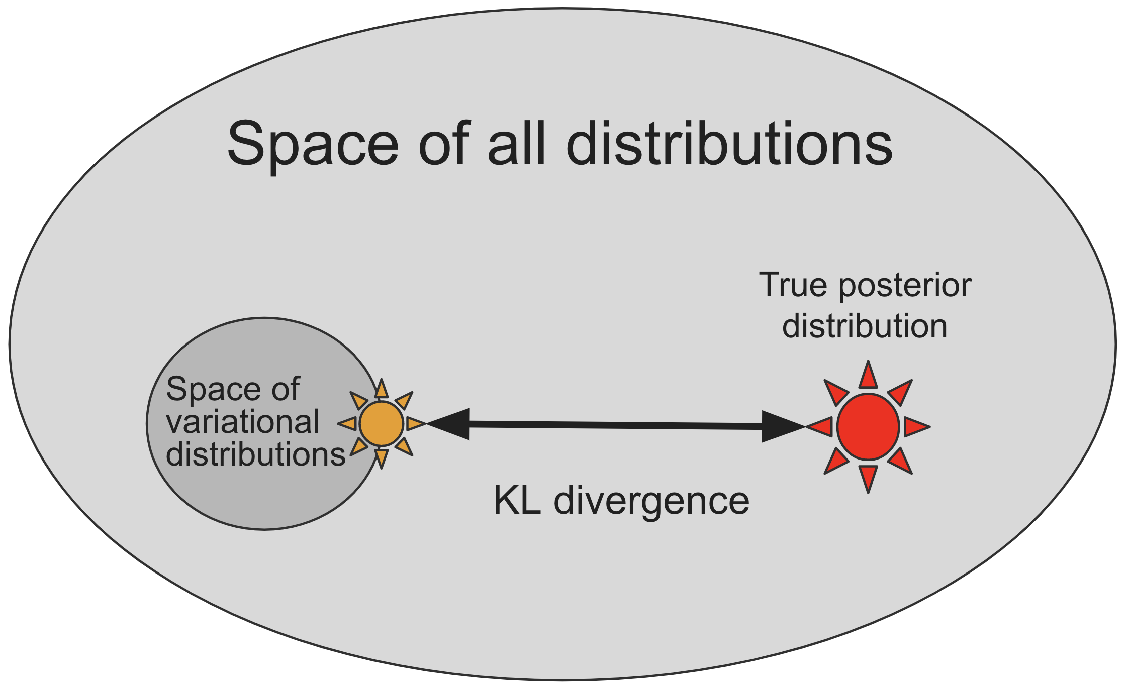
• Most distributions, especially Bayesian posterior distributions, too complex to represent directly
• In SVI, we define a smaller subspace/family, indexed by real-valued parameters $\phi$, of distributions $q_{\phi}({\bf z})$

that are by construction easy to sample from (e.g. family of gaussians)

• However, this family of distributions may not include the true posterior distribution $p_{\theta}({\bf z} | {\bf x})$
• SVI approximates the true posterior by searching the space of variational distributions

to find one that is most similar to the true posterior according to some measure of distance:

• Many different choices of distance measures between probability distributions! Which one should we choose?
• As in the figure, a theoretically appealing choice is the (non-negative) Kullback-Leibler divergence (KL divergence)

$$KL(q_{\phi}({\bf z}) || p_{\theta}({\bf z} | {\bf x})):= \mathbb{E}_{q_\phi(z)}\left [log\frac{q_\phi(z)}{p_\theta(z|x)}\right]$$

• Problems raised by this:

1. Computing this $KL$ directly requires knowing the true posterior $p_{\theta}({\bf z} | {\bf x})$ ahead of time, which defeats the purpose.
2. This would require the integral over the evidence $p_\theta(x)$ we are trying to avoid!
3. Also, we want to minimize this distance, which is even harder!

• Solution: It turns out we can rewrite this $KL$ as the difference between

the log evidence $\log p_\theta(x)$, which does not depend on $q_{\phi}$,
and a tractable term called the *evidence lower bound (ELBO)*: $$KL = log\;evidence - ELBO$$

• For the very short derivation see e.g. this blog post
• Just from the eqn. above, and since $KL\geq0$, some practical things follow:

1. The ELBO really is a lower bound of the (log) evidence:

$$ELBO = log\;evidence - KL \Rightarrow ELBO \leq log\;evidence$$

2. So if we take (stochastic) gradient steps to maximize the ELBO, we will also be pushing the log evidence higher (in expectation)!
3. Maximizing the ELBO will produce the same solution as minimizing the original KL-divergence!

Evidence Lower Bound (ELBO)

• The ELBO, which is a function of both $\theta$ and $\phi$, is defined as an expectation w.r.t. to samples from the guide:

$$\mathcal{L}(\theta,\phi;x) := \mathbb{E}_{q_{\phi}({\bf z})} \left [ \log \frac{p_{\theta}({\bf x}, {\bf z})}{q_{\phi}({\bf z})} \right] = \int_Z q_\phi({\bf z}) (\log p_{\theta}({\bf x}, {\bf z}) - \log q_{\phi}({\bf z})) d{\bf z} $$

• We can compute the log probabilities inside the expectation. (Because this time we avoid the posterior!)
• Since we picked a parametric distribution we can sample from as our guide, we can compute Monte Carlo estimates of the ELBO!
• For a fixed $\theta$, as we take steps in $\phi$ space that increase the ELBO, we move the guide toward the posterior.
• Actually, we take gradient steps in both $\theta$ and $\phi$ space simultaneously:
• SVI.step() does:

1. a step in 𝜙−space that moves the guide closer to the posterior.
2. a step in 𝜃−space that moves the posterior closer to the guide.

$\Rightarrow$ The guide and model play chase.
Despite the moving target, this optimization problem can be solved well enough for many different problems.

So at high level variational inference is easy:

1. Define a guide.
2. Compute gradients of the ELBO.

Pyro Primitives

Probabilistic models in Pyro are specified as Python functions, e.g. model(*args, **kwargs),
that generate observed data from latent variables using special primitive functions
whose behavior can be changed by Pyro's internals depending on the high-level computation being performed.

Specifically, the different mathematical pieces of model() and guide() are encoded via the mapping:

1. latent random variables $z$ $\Longleftrightarrow$ pyro.sample
2. observed random variables $x$ $\Longleftrightarrow$ pyro.sample with the obs keyword argument (model only)
3. learnable parameters $\theta$ $\Longleftrightarrow$ pyro.param (attribute of pyro.nn.module)
4. plates (iid copies) $\Longleftrightarrow$ pyro.plate context managers

Pyro's "guide" programs

• Just like the model(...), a guide is encoded as a Python program guide(...) that contains pyro.sample and pyro.param statements.
• Pyro allows guides to contain arbitrary python code!
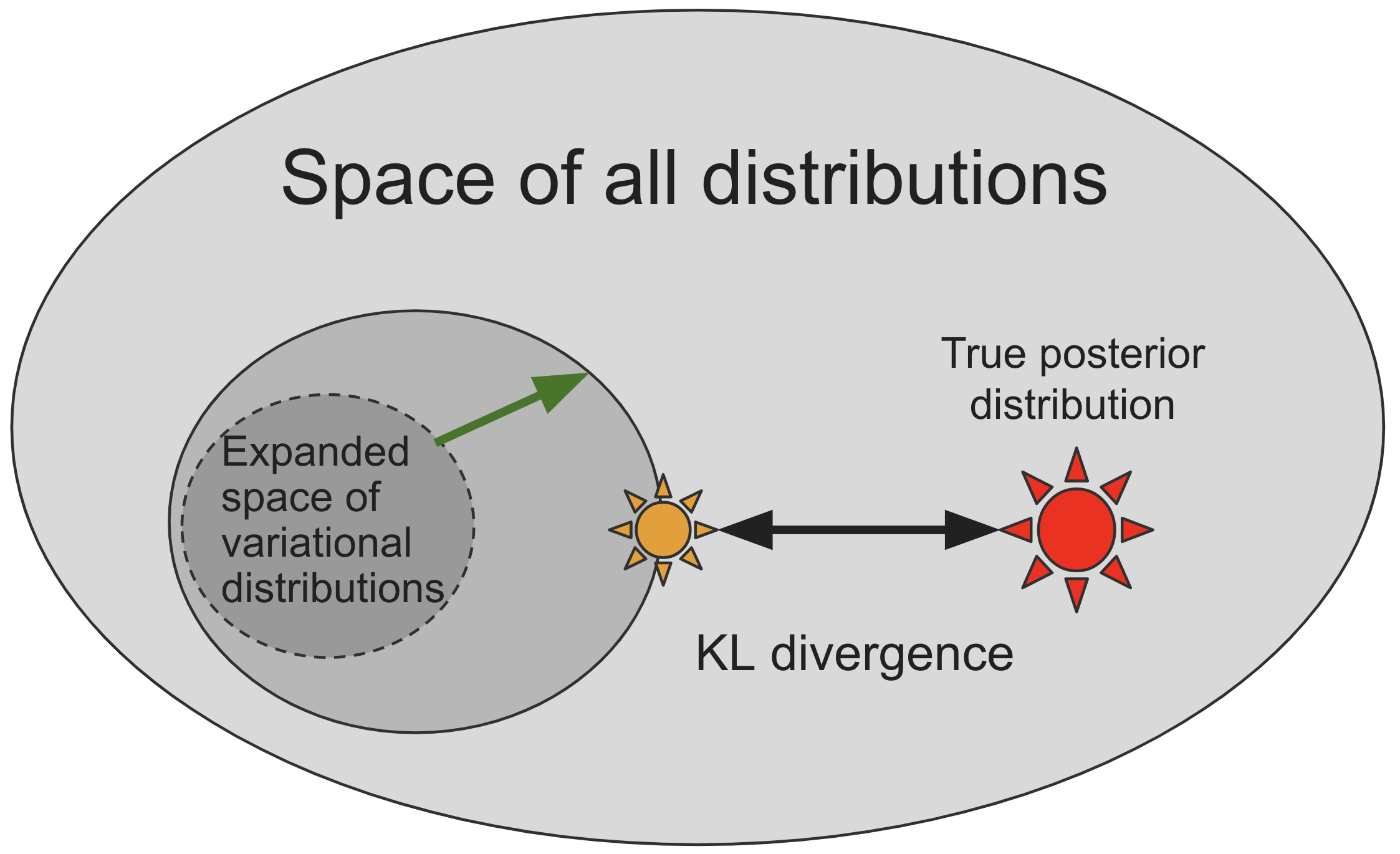
• This opens up the possibility of writing guide families that capture more of the problem-specific structure of the true posterior
• This allows us to encode our knowledge about the posterior and potentially expand the search space:

Restrictions on guides

• Since the guide approximates the posterior $p_{\theta_{\rm{max}}}({\bf z} | {\bf x})$, it needs to provide a valid joint probability density over all the latent random variables z in the model
• When random variables are specified in Pyro with the primitive statement pyro.sample() the first argument is the name of the random variable
• These names will be used to align the random variables in the model and guide.
• To be very explicit, if the model contains a random variable z_1 without the obs= keyword,

def model():
    pyro.sample("z_1", ...)

then the guide MUST have a matching sample statement

def guide():
    pyro.sample("z_1", ...)

The distributions used in the two cases can be different, but the names must line-up 1-to-1.

• The guide may not contain observed data (obs= keyword), since the guide needs to be a properly normalized distribution so that it is easy to sample from!
• Furthermore, model() and guide() should take the same arguments
• Problem: Writing out guides by hand is difficult and tedious
• Solution: Use *autoguides*, which automatically generate common guide families given arbritrary models. See pyro.infer.autoguide and below.

Pyro Summary

• Automatic generation of good default guides automatically for abritrary stochastic model() functions
• Pyro contains powerful high level abstractions that change the behavior of the model and guide
• without having to reimplement model and guide.
• This also means we can change between Pyro's various inference algorithms on the fly or implement one.
• Most of the other inference algorithms don't even need a guide.
• For many, many more examples, see the Pyro examples and Docs & Contributed Examples.

Pyro Example: Variational Autoencoder (VAE)

• Before we turn to BNNs, let's briefly look at what a more typical deep model with latent variables looks like in Pyro.
• The most general class of such models may be the Variational Autoencoder (VAE).
• Introduced by Kingma & Welling (2013), the VAE s were the first deep models which reduced the variance in the gradient of the ELBO sufficiently.

Please note:

• This section shows how one would write a guide explicitly
• Therefore, it won't necessarily be shorter than a PyTorch VAE implementation
• But keep in mind Pyros abovementioned advantages.
• The below model and comments are taken from the Pyro VAE Tutorial.

# ---- VAE example on MNIST's handwritten digit data ----

from vae import Encoder, Decoder # appropriate torch.nn.Modules

class VAE(nn.Module):
    def __init__(self, z_dim=50, hidden_dim=400, use_cuda=False):
        super().__init__()
        # create the encoder and decoder networks
        self.encoder = Encoder(z_dim, hidden_dim)
        self.decoder = Decoder(z_dim, hidden_dim)

        if use_cuda:
            # calling cuda() here will put all the parameters of
            # the encoder and decoder networks into gpu memory
            self.cuda()
        self.use_cuda = use_cuda
        self.z_dim = z_dim

    # define the model p(x|z)p(z)
    def model(self, x):
        # register PyTorch module `decoder` with Pyro
        pyro.module("decoder", self.decoder)
        
        # this context makes the samples in the batch independent:
        with pyro.plate("data", x.shape[0]):
            
            # setup parameters for gaussian prior p(z)
            z_loc = x.new_zeros(torch.Size((x.shape[0], self.z_dim)))
            z_scale = x.new_ones(torch.Size((x.shape[0], self.z_dim)))
            
            # sample from prior (value will also be sampled by guide when computing the ELBO)
            z = pyro.sample("latent", dist.Normal(z_loc, z_scale).to_event(1))
            # dist.to_event(n) declares the n rightmost dimensions as being RVs, the rest are batch dimensions
            
            # decode the latent code z
            img = self.decoder(z)
            
            # score against actual images 
            # (results in reconstruction loss = log likelihood for decoder)
            pyro.sample("obs", dist.Bernoulli(img).to_event(1), obs=x.reshape(-1, 784)) # bernoulli to sample black/white
            
            # return the img only so that we can visualize it later
            return img
        
VAE.model = model

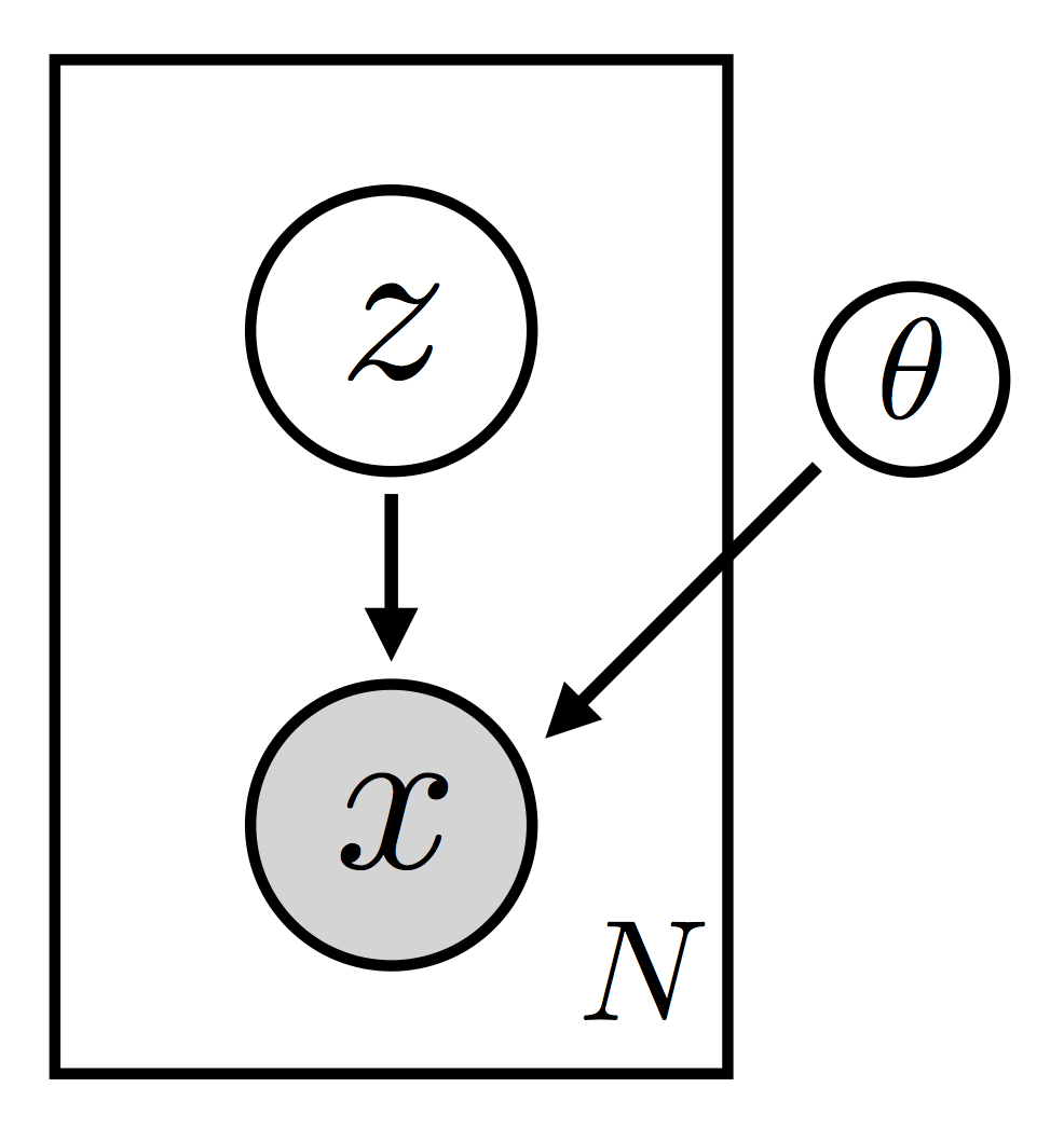
VAE.model(x)

• The first thing we do inside of model() is to register the (previously instantiated) decoder module with Pyro.
• Note that we give it an appropriate (and unique) name.
• This call to pyro.module lets Pyro know about all the parameters inside of the decoder network.
• Next we setup the hyperparameters for our prior, which is just a multivariate standard normal.

Note that:

• we designate independence in the batch dimension (i.e. the leftmost dimension) via pyro.plate.
• The call .to_event(1) when sampling from the latent z tells pyro the rightmost dimension is multivariate. See Pyros Tensor Shapes tutorial for more details.

VAE.model(x) as a graphical model:

    # define the guide (i.e. variational distribution) q(z|x)
    def guide(self, x):
        # register PyTorch module `encoder` with Pyro
        pyro.module("encoder", self.encoder)
        with pyro.plate("data", x.shape[0]):
            # use the encoder to get the parameters used to define q(z|x)
            z_loc, z_scale = self.encoder(x)
            
            # sample the latent code z
            pyro.sample("latent", dist.Normal(z_loc, z_scale).to_event(1))

VAE.guide = guide

VAE.guide(x)

• Just like in the model, we first register the PyTorch module we're using (namely encoder) with Pyro.
• We take the mini-batch of images x and pass it through the encoder.
• Then, using the parameters output by the encoder network we use the normal distribution to sample a value of the latent for each image in the mini-batch.
• Crucially, we must use the same name for the latent random variable as we did in the model: 'latent'.

VAE.guide(x) as a graphical model:

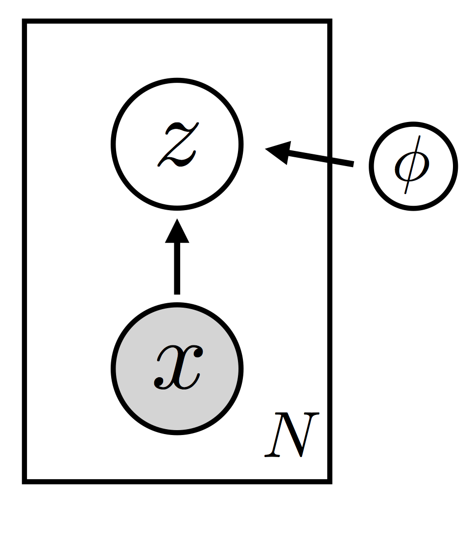
• From the implementation and the graphical model we can see that the guide depends on $x$, i.e. it's $q_\phi(z|x)$.

Now that we've defined the full model and guide inside our torch.nn.Module "VAE" we can setup inference:

# preliminaries 

from utils import make_loaders_mnist
from vae import train
from vae import evaluate

# Run options
smoke_test = True # short run
LEARNING_RATE = 1.0e-3

# Run only for a single iteration for testing
NUM_EPOCHS = 1 if smoke_test else 100
TEST_FREQUENCY = 5

# load MNIST
train_loader, test_loader = make_loaders_mnist(
    batch_size=32,
    use_cuda=USE_CUDA
)

# clear pyro's global parameter store
pyro.clear_param_store()

To set up the SVI, all we need to do is:

# setup the VAE
vae = VAE(
    z_dim=10,
    hidden_dim=40,    
    use_cuda=USE_CUDA
)

# setup the optimizer
optimizer = pyro.optim.Adam({"lr": LEARNING_RATE}) # pyro.optim wraps torch.optim

# setup the stochastic variational inference algorithm
svi = pyro.infer.SVI(vae.model, vae.guide, optimizer, loss=pyro.infer.Trace_ELBO())

# training
train_elbo = []
test_elbo = []

# training loop
for epoch in range(NUM_EPOCHS):
    # simply calls svi.step(batch) as train loop
    total_epoch_loss_train = train(svi, train_loader, use_cuda=USE_CUDA)
    train_elbo.append(-total_epoch_loss_train)
    print("[epoch %03d] average training loss: %.4f" % (epoch, total_epoch_loss_train))

    if epoch % TEST_FREQUENCY == 0:
         # simply calls svi.evaluate_loss(batch) as test loop
        total_epoch_loss_test = evaluate(svi, test_loader, use_cuda=USE_CUDA)
        test_elbo.append(-total_epoch_loss_test)
        print("[epoch %03d] average test loss: %.4f" % (epoch, total_epoch_loss_test))

Pyro Example: Model Evaluation

(Bayesian model evaluation with posterior predictive checks)
(Sometimes called sanity check)

• Can easily approximate the posterior predictive distribution using our guide obtained from SVI:

$$p_{\theta}(x' | {\bf x}) = \int \! p_{\theta}(x' | {\bf z}) p_{\theta}({\bf z} | {\bf x})\; d{\bf z} \approx \int \! p_{\theta}(x' | {\bf z}) q_{\phi}({\bf z} | {\bf x})\; d{\bf z}$$

1. Simply draw a sample ${\hat {\bf z}} \sim q_{\phi}({\bf z})$ from the guide
2. Then sample new data point $x' \sim p_{\theta}(x | {\hat {\bf z}})$, as if we had replaced the prior with our guide.

# plot example images

row = 12
column = 3
plt.figure(figsize=(20,5))

mock_input = torch.zeros([1, 784]) # does not matter, check VAE.model

if USE_CUDA:
    mock_input = mock_input.cuda()

for i in range(1, row * column +1):
    plt.subplot(column, row, i) 

    # get img from the model.
    # model samples internally and practically ignores mock_input
    sample_img = vae.model(mock_input) # p(img|z)p(z) 
    
    img = sample_img[0].view(28, 28).cpu().data.numpy()
    plt.xticks([])
    plt.yticks([]) 
    plt.imshow(img, cmap="gray")

# time for a coffee pause? :)

Bayesian Neural Networks

• Now that we've discussed SVI in general, it is straightforward to apply it to the case of BNNs.
• Instead of learning model weights $\theta$ to parameterize distributions of latent variables $z$,
• we are now going to be bayesian about the model weights themselves,
• i.e. in all above formulae we reinterpret the variables:

1. ${\bf z}$ now designates the (already learned) neural network model weights
2. $\theta$ are now the learnable distribution parameters (usually: (multivariate) scale and location of gaussians)

The training workflow for BNNs is that

1. We take a given neural network, usually pretrained using MLE,
2. We replace all weights with gaussians priors,
3. Then guide the network with a gaussian guide with means initialized to the pretrained weights,
4. We learn the parameters og the guide only.

Usually we fix the means to the pretrained weights and only learn the variances.

For a minibatch of data, the ELBO now takes on the form:

$$ELBO = -logq_\phi(z)+logp_\theta(z)+\frac{1}{n}\sum_{i=1}^nlogp_\theta(x_i|z)$$

where $z\sim q_\phi(z)$ is drawn ahead of time.

according to Weight Uncertainty in Neural Networks (Blundell et al., 2015). (This is a Monte Carlo Estimate of the ELBO with 1 Sample)

Bayesian ResNet in Pyro

• Theoretically, it is straightforward to adapt a given deep neural maximum likelihood estimator to be a BNN.
• Let's see how we would do this in Pyro, practically.
• Code adapted from Appendix B of the TyXe Paper

# preliminaries

# dataset helper functions
from utils import make_loaders_bnns, make_net

dataset = "cifar10"
model_name = "resnet18"
pretrained = False # usually, start with a net pretrained using MLE!

# load cifar data
train_loader, test_loader, _ = make_loaders_bnns(
    dataset, "./data", 32, 32, False, False 
)

# take an existing net:
resnet: torch.nn.Module = make_net(dataset, model_name, pretrained=pretrained)
# make_net only reshapes final layer of torchvision.models.model_name()

# initialize gaussian means using these:
pretrained_weights = resnet.state_dict()

# convert model to pyro module inplace
pyro.nn.module.to_pyro_module_(resnet)

Now we have to make choices for the following three Bayesian components:

1. Prior - Our Prior Belief $p_\theta({\bf z})$ about the weights.
2. Likelihood - The Likelihood of our Training Data $p_\theta({\bf x}|{\bf z})$. Together with the Prior this constitutes the Model.
3. Guide - The Variational Distribution $q_\phi({\bf z}|{\bf x})$.

For each of these three components, we

• Pick the family of distributions the particular object may belong to.
• Initialize the distribution's parameters.

1. Prior

We pick standard normals as our prior belief $p_\theta(weights)$ about the weights.

for m in resnet.modules():
    # replace weights and biases of 
    # fully connected and convolutional modules
    # (do not be bayesian about batchnorms)
    if isinstance(m, (nn.Linear, nn.Conv2d)):
        # PyroSample Modules sample on their forward pass,
        m.weight = pyro.nn.PyroSample(
            dist.Normal(
                torch.zeros_like(m.weight),
                torch.ones_like(m.weight)
            ).to_event()
        )
        if m.bias is not None:
            m.bias = pyro.nn.PyroSample(
                dist.Normal(
                    torch.zeros_like(m.bias),
                    torch.ones_like(m.bias)
                ).to_event()
            )

2. Likelihood

We define the likelihood $p_\theta(data|weights)$ by defining our model $p_\theta(data|weights) * p(weights)$, i.e.
p(data | weights) * p(weights)
= likelihood * prior
= joint distribution

def model(x, y=None):
    logits = resnet(x) # forward samples from prior
    
    # define the likelihood 
    # p(data | weights)
    with pyro.plate("data_plate", x.shape[0]):
        # context for IID data points in batch
        
        # log likelihood reconstruction loss
        pyro.sample("data", dist.Categorical(logits=logits), obs=y)
        
        # return for prediction/testing only:
        return logits

3. Guide

We decide that the guide $q_\phi(weights)$ should be gaussian.
In this case, the use of AutoNormal leads to diagonal covariance, i.e. independent weights.
This is called Mean-Field assumption and drastically reduces training time.

guide = pyro.infer.autoguide.AutoNormal(
    model,
    init_scale=1e-4, # initialize the variances uniformly (vars=phi above)
    init_loc_fn=pyro.infer.autoguide.init_to_value(
        values=pretrained_weights
    ) # init gauss means to pretrained weights
)

# an optimizer can be taken from pyro.optim (wrapper around torch.optim API)
optim = pyro.optim.Adam({"lr": 1e-3})

# set up stochastic variational inference
svi = pyro.infer.SVI(
    model,
    guide,
    optim,
    pyro.infer.Trace_ELBO() # objective function
)

# training

# fit the BNN
num_epochs = 1
first_n_batches_train = 20

for _ in range(num_epochs):
    for i, (x, y) in enumerate(iter(train_loader)):
        if i > first_n_batches_train:
            break
            
        # 1. forward guide(x,y), memorize sampled weight values
        # 2. forward model(x,y), using memorized values
        # 3. compute the elbo
        # 4. elbo.backward() # updates guide
        svi.step(x, y)

# prediction
def make_prediction(model, guide, x, y):
    trace = pyro.poutine.trace(guide).get_trace(x) # memorize sampled weight values of guide
    logits = pyro.poutine.replay(model, trace=trace)(x) # use sampled weight values of guide
    predictions = logits.argmax(-1)

    acc = ((predictions == y).sum()/y.shape[0]).item()
    print(f"Batch acc = {acc}")


first_n_batches_test = 10

test_predictions = [make_prediction(model, guide, x, y) for i, (x, y) in enumerate(test_loader) if i < first_n_batches_test]

There are a few things to note here:

• we had to touch the torch.nn.Module and use our knowledge of it
• we had to have quite a bit of knowledge of pyro's internals
• we do not have access to variance reduction techniques typically used in BNN training
• testing is unnecessarily complicated. According to the TyXe Paper (Appendix B), this may be because

„Pyro was primarily designed" for a „smaller-scale Bayesian Workflow"
where one is interested in „modelling and making inferences on a given dataset
rather than predicting on held-out test data“.

In the next section, we will see that the Pyro-based BNN library TyXe solves these problems:
TyXe users only have to have familiarity with pytorch, and minimal knowledge of the BNN workflow.

Bayesian ResNet in TyXe

TyXe (Ancient greek: goddess of chance) is built ontop of Pyro and was released in 2021 as
a BNN library aimed at hiding away most of what we had to do manually for our bayesian resnet above.

# first some more imports:
import os
import contextlib
import functools
from typing import List, Optional

import tyxe # bnn library ontop of pyro

from utils import make_loaders_bnns, make_net

In Tyxe, the following short code is equivalent to our previous Bayesian ResNet:

# take an existing torch.nn.Module:
resnet: torch.nn.Module = make_net("cifar10", "resnet18", pretrained=False)

# setup bnn:
prior = tyxe.priors.IIDPrior(dist.Normal(0,1), expose_all=False, hide_module_types=(nn.BatchNorm2d,))
likelihood = tyxe.likelihoods.Categorical(len(train_loader))
guide = functools.partial(
    tyxe.guides.AutoNormal, 
    train_loc=False,
    init_loc_fn=tyxe.guides.PretrainedInitializer.from_net(resnet)
)
bnn = tyxe.VariationalBNN(resnet, prior, likelihood, guide)

# train bnn
# (execute with care; very compute intensive, may be too much for cpu!)
# bnn.fit(train_loader, optim=pyro.optim.Adam({"lr":1e-3}), num_epochs=1, device="gpu" if USE_CUDA else "cpu")

TyXe Options

As you can see, users technically don't need to be intricately familiar with Pyro to use TyXe.
With TyXe we've reached a level of abstraction appropriate for BNNs,
so let's look at some more typical training setups in TyXe.
First, let's get the standard Hyperparameters out of the way:

# Standard Hyperparameters first ...

# MODEL
architecture: str = "resnet18"
dataset: str = "cifar10"
pretrained: bool = False
mock_dataset: bool = False

# DATA
train_batch_size: int = 10
test_batch_size: int = 10
num_epochs: int = 1
test_samples: int = 20

# MISC
root: str = os.environ.get("DATASETS_PATH", "./data")
seed: int = 42
output_dir: Optional[str] = None

# OPTIMIZER
lr: float = 0.001 # initial learning rate
milestones: Optional[List[int]] = None # epochs at which to do scheduler step
gamma: float = 0.1 # scheduler step factor

resnets = [n for n in dir(torchvision.models) if (n.startswith("resnet") or n.startswith("wide_resnet")) and n[-1].isdigit()]
assert architecture in resnets, architecture

datasets = ["cifar10", "cifar100", "mnist"]
assert dataset in datasets, dataset

# Some BNN Hyperparameters:

inference: str = "mean-field"
local_reparameterization: bool = False # important: variance reduction for gradients!
flipout: bool = False # important: variance reduction for gradients!
max_guide_scale: float = 0.1 # to prevent underfitting: clamp learned variance
rank: int = 10 # low rank setting for inference == "last-layer-low-rank"
scale_only: bool = False # train variance only, leaving means at pretrained values

# More comments on these inference options in the section 'guide' below
inference_options = [
    "mle", # maximum likelihood estimation: weights = argmax p(data|weights)
    "map", # maximum a posteriori inference: weights = argmax p(data|weights)*p(weights)
    "mean-field", # svi with autonormal guide (diagonal covariance)
    "last-layer-mean-field", # svi for last layer only, autonormal guide and diagonal covariance
    "last-layer-full", # svi for last layer only, autonormal guide and FULL covariance
    "last-layer-low-rank" # svi for last layer only, low rank
]
assert inference in inference_options, inference

Initialize our Dataset and Model

• arbitrary pytorch datasets and models work
• it is straightforward to integrate TyXe into any existing Pytorch workflow
• since we just start out with any torch.nn.Module and never touch its internals!

# ----- set up pyro & torch -----
use_cuda = torch.cuda.is_available()
device = torch.device("cuda" if USE_CUDA else "cpu")

# ----- set up dataset and model -----
train_loader, test_loader, ood_loader = make_loaders_bnns(
    dataset, root, train_batch_size, test_batch_size, use_cuda, mock_dataset
)

net: torch.nn.Module = make_net(dataset, architecture, pretrained=pretrained).to(device)

Set up ResNet to be Bayesian using TyXe

Once again, to set up a BNN we need to make choices for the Prior, Likelihood and Guide.

1. Likelihood

The Likelihood of our Training Data $p_\theta({\bf x}|{\bf z})$.
The support of the distribution must be equal in size to the number of training samples.

# tyxe.likelihoods includes:

# Bernoulli
# Categorical
# HeteroskedasticGaussian
# HomoskedasticGaussian

likelihood = tyxe.likelihoods.Categorical(len(train_loader.sampler))

# uncomment for documentation:
# tyxe.likelihoods.HeteroskedasticGaussian?

2. Guide

• The choice of the guide is where most of our flexibility lies.
• TyXe's BNNs expect a partially initialized Autoguide function, either from Pyro or TyXe.
• Let's go through some typical options, which are all
• practical approximations to SVI on the full model with full gaussian covariances
• which is far too expensive.

Instead of SVI on the full model with full gaussian covariances, we will do one of:

1. Maximum Likelihood: Just let the guide be None.
2. Maximum a posteriori Inference: Because of Math, we can just use Delta Distributions as guides for this.
3. Mean Field: Does SVI on full model with Independent Gaussians, i.e. Diagonal Covariances

($\Rightarrow Training\in\mathcal{O}(\#params)$ instead of $\mathcal{O}(\#params^6)$ - Oxford Blog Post. According to the post & paper, the Diagonal Covariances are good enough especially for deeper models.) 4. Last Layer: Often only the last layer of a Big Conv Net is tuned with SVI

See the Paper for a comparison of these methods both on CIFAR's test set and Out Of Domain data.

if inference == "mle":
    # do maximum likelihood estimation
    test_samples = 1
    guide = None

if inference == "map":
    # maximum a posteriori inference 
    test_samples = 1
    guide = functools.partial(
        pyro.infer.autoguide.AutoDelta, # deterministic weights
        init_loc_fn=tyxe.guides.PretrainedInitializer.from_net(net)
    )

if inference == "mean-field":
    # SVI with diagonal covariances
    guide = functools.partial(
        tyxe.guides.AutoNormal,
        init_loc_fn=tyxe.guides.PretrainedInitializer.from_net(net),
        init_scale=1e-4,
        max_guide_scale=max_guide_scale, # prevent underfitting
        train_loc=not scale_only # train gaussian means?
    ) 

if inference.startswith("last-layer"):
    # usually only done for pretrained network:
    # if not pretrained:
    #    raise ValueError("Asked to do last-layer inference, but no pre-trained weights were provided.")
    
    # turning parameters except for last layer in buffers to avoid training them
    # this might be avoidable via poutine.block
    for module in net.modules():
        if module is not net.fc:
            for param_name, param in list(module.named_parameters(recurse=False)):
                delattr(module, param_name)
                module.register_buffer(param_name, param.detach().data)

    if inference == "last-layer-mean-field":
        guide = functools.partial(
            tyxe.guides.AutoNormal, 
            init_loc_fn=tyxe.guides.PretrainedInitializer.from_net(net),
            init_scale=1e-4
        )
        
    elif inference == "last-layer-full":
        guide = functools.partial(
            pyro.infer.autoguide.AutoMultivariateNormal,
            init_loc_fn=tyxe.guides.PretrainedInitializer.from_net(net),
            init_scale=1e-4
        )
        
    elif inference == "last-layer-low-rank":
        guide = functools.partial(
            pyro.infer.autoguide.AutoLowRankMultivariateNormal,
            rank=rank,
            init_loc_fn=tyxe.guides.PretrainedInitializer.from_net(net),
            init_scale=1e-4
        )

Pyro's Automatic Guide Families:
['AutoCallable', 'AutoContinuous', 'AutoDelta', 'AutoDiagonalNormal', 'AutoDiscreteParallel', 'AutoGuide', 'AutoGuideList', 'AutoIAFNormal', 'AutoLaplaceApproximation', 'AutoLowRankMultivariateNormal', 'AutoMultivariateNormal', 'AutoNormal', 'AutoNormalizingFlow']
TyXe's Automatic Guide Families:
['AutoNormal']

print("Pyro's Automatic Guide Families:")
print([g for g in dir(pyro.infer.autoguide) if g.startswith("Auto")])

print("TyXe's Automatic Guide Families:")
print([g for g in dir(tyxe.guides) if g.startswith("Auto")])

# uncomment for documentation:
# pyro.infer.autoguide.AutoDelta?

3. Prior

# it is standard practice to not be bayesian about batchnorm modules:
prior_kwargs = {
    "expose_all": False, # do not treat all nn.Modules with pyro 
    "hide_module_types": (nn.BatchNorm2d,) # specifically, ignore batchnorms
}

# our choice of guide impacts how we need to initialize the Prior:
if inference == "mle":
    # we dont want a prior for maximum likelihood estimation
    prior_kwargs["hide_all"] = True
    
elif inference.startswith("last-layer"):
    # only be bayesian about the final, fully connected layer
    del prior_kwargs['hide_module_types']
    prior_kwargs["expose_modules"] = [net.fc]
    
prior = tyxe.priors.IIDPrior(
    dist.Normal(
        torch.zeros(1, device=device),
        torch.ones(1, device=device)
    ),
    **prior_kwargs
)

print("TyXe's Available Prior Distributions:")
print([p for p in dir(tyxe.priors) if p.endswith("Prior")])

# uncomment for documentation:
# tyxe.priors.IIDPrior?

TyXe's Available Prior Distributions:
['DictPrior', 'IIDPrior', 'LambdaPrior', 'LayerwiseNormalPrior', 'Prior']

Thats it! We're ready to set up our BNN:

# Finally set up our VariationalBNN!
bnn = tyxe.VariationalBNN(
    net, prior, likelihood, guide
)

# uncomment for documentation:
# bnn?

Variance Reduction

• One very important thing for successful SVI via gradient descent we haven't touched upon is gradient variance reduction.
• The most classical example: reparameterization trick (introduced in VAE paper, described here)
• Though Pyro provides many variance reduction techniques and tutorials,
• TyXe provides some context managers specific to its BNNs:

# gradient variance reduction techniques:
if local_reparameterization:
    if flipout:
        raise RuntimeError("Can't use both local reparameterization and flipout, pick one.")
    train_context = tyxe.poutine.local_reparameterization
    # turns each
    # torch.distributions.Normal(loc, scale).sample() (gradient w.r.t. loc, scale is stochastic)
    # into
    # loc + scale * torch.distributions.Normal(0, 1).sample() (gradient w.r.t. loc, scale is deterministic) 
elif flipout:
    # usually: use one sampled weight for entire minibatch
    # flipout: efficiently sample pseudo-independent weights along the minibatch dimension
    train_context = tyxe.poutine.flipout
else:
    train_context = contextlib.nullcontext

Optimizer

# pyro-specific: optimizer must come from pyro.optim
if milestones is None:
    optim = pyro.optim.Adam({"lr": lr})
else:
    optimizer = torch.optim.Adam
    optim = pyro.optim.MultiStepLR({"optimizer": optimizer, "optim_args": {"lr": lr}, "milestones": milestones, "gamma": gamma})

print("All typical pytorch optimizers & schedulers are supported by pyro.optim:")
print([opt for opt in dir(pyro.optim) if "_" not in opt and opt[0] == opt[0].upper()])

All typical pytorch optimizers & schedulers are supported by pyro.optim:
['ASGD', 'Adadelta', 'Adagrad', 'AdagradRMSProp', 'Adam', 'AdamW', 'Adamax', 'ChainedScheduler', 'ClippedAdam', 'ConstantLR', 'CosineAnnealingLR', 'CosineAnnealingWarmRestarts', 'CyclicLR', 'DCTAdam', 'ExponentialLR', 'LambdaLR', 'LinearLR', 'MultiStepLR', 'MultiplicativeLR', 'NAdam', 'OneCycleLR', 'PyroLRScheduler', 'PyroOptim', 'RAdam', 'RMSprop', 'ReduceLROnPlateau', 'Rprop', 'SGD', 'SequentialLR', 'SparseAdam', 'StepLR']

Evaluation logic

# tyXe-specific: evaluation and logging done after every epoch:
def callback(
        b: tyxe.VariationalBNN, # bnn
        i: int, # epoch number
        avg_elbo: float # mean elbo this epoch
    ):
    avg_err, avg_ll = 0., 0.
    
    for x, y in iter(test_loader):t
        err, ll = b.evaluate(x.to(device), y.to(device), num_predictions=test_samples)
        avg_err += err / len(test_loader.sampler)
        avg_ll += ll / len(test_loader.sampler)
        
    print(f"ELBO={avg_elbo}; test error={100 * avg_err:.2f}%; LL={avg_ll:.4f}")

Training

# ------ TRAIN THE MODEL ------
with train_context():
    bnn.fit(train_loader, optim, num_epochs, callback=callback, device=device)

That's it!

This notebook and its dependencies were assembled from, in rough order:

• Pyro/Examples/Intro
• Pyro/Examples/SVI_Intro
• Pyro/Examples/VAE
• TyXe Paper (Appendix B Pyro Example)
• TyXe Resnet Example