Uncertainty Quantification using Bayesian Neural Networks

---

BNN Slides from last time
Our goal: Understand how to express different sources of uncertainty using BNNs, for the task of regression.

Theory - Aleatoric & Epistemic Uncertainty

---

(Hüllermeier & Wagemann (2020))

Uncertainty quantified by some model fit to data can come from two sources:

1. ALEATORIC Spread/stochasticity/noise present in the data. Even with a perfect model, this uncertainty persists; it is IRREDUCIBLE.
2. EPISTEMIC Uncertainty about which model is appropriate for the data. With more data, this type of uncertainty is REDUCIBLE.

Useful Mnemonics:

• Aleatoric (Latin Alea: Dice): uncertainty due to data generated by dice-throw-like processes.
• Epistemic (Greek episteme: knowledge): uncertainty due to a lack of knowledge.

How to distinguish these two?

• There is no universal mathematical definition of these terms;
• It depends on the class of models.
• The presence of aleatoric uncertainty does NOT depend on the type of model, of course,
• But whether and how we can distinguish it from epistemic uncertainty does.

In Neural Networks

• Deterministic NNs (Maximum Likelihood Estimators) cannot quantify epistemic uncertainty.
• Bayesian NNs can quantify the epistemic uncertainty through the part of the output variance caused by the weight distribution.

NNs applied to Regression

In the case of regression, we typically use our neural network with weights $\theta$ to parameterize a Gaussian Likelihood over some space: $$p_\theta(y|x) = \mathcal{N}(\mu,\sigma^2)$$ That is, we construct the architecture to learn the two parameters of a Gaussian distribution.

$Math$

When we make predictions $\hat{Y}\sim p_\theta(y|x) = \mathcal{N}(\mu,\sigma^2)$,
by the Law of total Variance,

$$\underset{\text{predictive variance}}{\mathbb{V}\text{ar}[\hat{Y}]} = \underset{\text{aleatoric uncertainty}}{\mathbb{E}_{p_\theta}[\sigma^2]} + \underset{\text{epistemic uncertainty}}{\mathbb{V}\text{ar}_{p_\theta}[\mu]}$$

Code

Sampling the BNN's weights $N$ times for one batch $x$ of $B$ datapoints, and output dimensionality $D$:

mu, sigma = bnn(x) # each of shape [N, B, D]
predictions = Normal(mu, sigma).sample() # [N, B, D] 
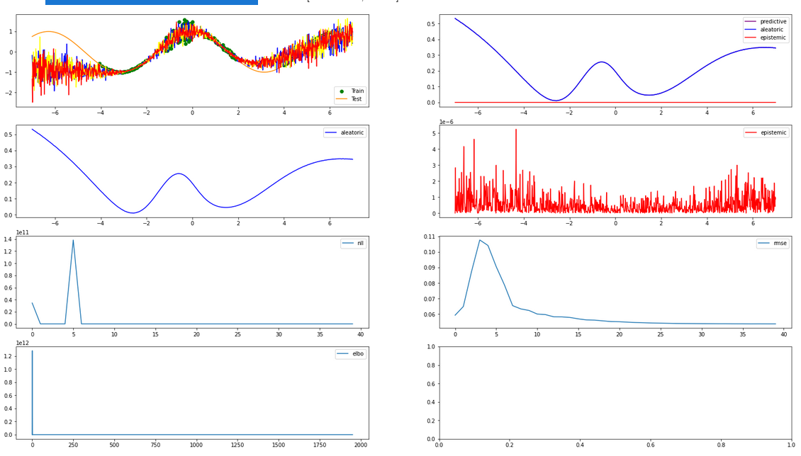
aleatoric = sigma.mean(dim=0) # [B, D]
epistemic = mu.var(dim=0) # [B, D]
predictive_variance = aleatoric + epistemic

We thus estimate the uncertainty of the prediction on each datapoint.

Practice - Regression UQ Experiments

---

0. Setup

If you installed the dependencies (including ipykernel) in a virtual environment,
select Kernel -> Change Kernel -> Environment Name.

# ========================= (Uncomment to) INSTALL REQUIREMENTS ==========================
# requires custom version of tyxe
# !git clone https://github.com/marvosyntactical/TyXe
# !python3 TyXe/setup.py

# ========================= IMPORTS ==========================

# built-in modules
from functools import partial
import itertools
import contextlib
from typing import Union, Optional, Dict, List
import warnings
warnings.simplefilter('once', UserWarning)

# logging/plotting
import math
from tqdm.notebook import tqdm
import matplotlib.pyplot as plt
%matplotlib inline

# Adjust to browser/screen as needed
big_w = 26; small_w = 10; ratio = 16/9
big_figsize = (big_w, big_w/ratio); small_figsize = (small_w, small_w/ratio)
# uncomment to globally control figure size of all figures:
# plt.rcParams['figure.figsize'] = big_figsize # globally control figure size

# neural networks
import torch
import torch.nn as nn
import torch.utils.data as data
from torch import Tensor

# bayesian inference
import pyro
import pyro.distributions as dist
from pyro.infer.mcmc.util import initialize_model

# bayesian neural networks
import tyxe

from synth_utils import plot, make_data

# ========================= SEED ==========================
seed = 906
pyro.set_rng_seed(seed)
torch.manual_seed(seed)

<torch._C.Generator at 0x7f70bc1098f0>

# ======================== DEVICE =========================
use_cuda = True
device = torch.device("cuda" if use_cuda and torch.cuda.is_available() else "cpu")

device, torch.cuda.is_available()

(device(type='cuda'), True)

1. Data

Next up, we synthesize some simple clusters of data to do regression on.

We will set the clusters up so that we have

• a simple function underlying the data
• gaps with no data (places of complete uncertainty)
• varying levels of inherent statistical noise, per cluster

# ========================= DATA SYNTHESIS =========================

shuffle = True
n_train = 400
mini_batch_size = 400
n_mini_batches = math.ceil(n_train/mini_batch_size) # batches per epoch

x_train, y_train, x_test, y_test = data_tuple = make_data(
    n_train,
    shuffle_train=shuffle,
    f=lambda x: x.cos(), # x.pow(3)/350, 
    # ===== TyXe Regression example data clusters:
    # x1 = torch.rand(50, 1) * 0.3 - 1
    # x2 = torch.rand(50, 1) * 1.2 + 0.5
    # ===== 2 Alternative Clusters 
    #fracs =  [  0.5,  0.5], # , 0.7], 
    #stds =   [ 0.2, 0.05], # , 0.01],
    #spreads =[  0.3,  1.2],
    #offsets =[ -1.0,  0.5],
    # ===== 4 Alternative Clusters 
    fracs =  [ 0.25,  0.25, 0.25,  0.25],
    stds =   [ 0.01,  0.25, 0.05,  0.01], # vertical
    spreads =[  2.1,   1.2,  1.4,   2.0], # horizontal
    offsets =[   -4.1,  -1.2,  0.5,   4.0],
)

dataset = data.TensorDataset(x_train, y_train)
loader = data.DataLoader(dataset, batch_size=mini_batch_size, pin_memory=use_cuda, shuffle=shuffle)

Visualisation

Let's see what the Clusters look like.

# ========================= DATA VISUALIZATION =========================

fig, ax = plt.subplots(figsize=small_figsize)
ax.scatter(x_train.squeeze(), y_train, color="green", label="Train")
ax.plot(x_test.squeeze(), y_test, color="darkorange", label="Test")
plt.legend()

<matplotlib.legend.Legend at 0x7f7056ce7940>

2. Hyperparameters

2.0 Neptune Logging

# ============================================= NEPTUNE LOGGING ==========================================================

monitor = True # log to neptune? install + put api key in file as described in preprocessing.init_neptune
neptune_user = "halcyon"
neptune_project = "bnn-synthetic"

if monitor:
    import neptune.new as neptune
    from preprocessing import init_neptune

2.1 Inference: Variational Bayesian or MCMC?

# ========================= INFERENCE SETTINGS =========================
inference = "svi" # 'mcmc', 'svi', "mle", "map"
variational_infs = {"svi", "mle", "map"}

# -------------- hyperparameters that are independent of the kind of inference ----------
reparameterize = True # will not be done for MCMC prediction
heteroskedastic = True # use an architecture that also learns a data dependent standard deviation? Otherwise use same standard deviation everywhere.
n_test_samples = 3 # samples drawn for visualisation

2.2 Architecture

We use a simple feedforward architecture with a Tanh() nonlinearity in all experiments.

It is however dependent on the kind of likelihood we chose:

• Homoskedastic: Let the network only learn an x-dependent mean, and train a non-x-dependent standard deviation outside of the PyTorch network.
• Heteroskedastic: Let the network learn both x-dependent mean and standard deviation.

# ========================= NETWORK DEFINITION =========================

class FF(nn.Module):
    def __init__(self, dim=50, heteroskedastic=False, min_scale=1e-4):
        """
        >>> net = FF()  # corresponds to:
        >>> net = nn.Sequential(nn.Linear(1, 50), nn.Tanh(), nn.Linear(50, 1))
        """
        super().__init__()
        
        self.fc1 = nn.Linear(1, dim)
        self.tanh = nn.Tanh()

        self.loc_head = nn.Linear(dim, 1)
        
        self.heteroskedastic = heteroskedastic
        if self.heteroskedastic:
            self.scale_head = nn.Linear(dim, 1)
            # NOTE: used to constrain variance to be > 0 and possibly smaller than some value
            self.scale_nonlinearity = lambda s: s.clamp(min=1e-6, max=max_likelihood_scale)
            self.min_scale = min_scale

    def forward(self, x):

        x = self.fc1(x)
        x = self.tanh(x)
            
        mean = self.loc_head(x)
        
        if not self.heteroskedastic:
            return mean
        else:
            scale = self.scale_head(x)
            scale = self.scale_nonlinearity(scale)
            # tyxe.likelihoods.HeteroskedasticGaussian expects network output to be 
            # a concatenation of mean (no constraint) and scale (> 0) along last (hidden) dimension
            mean_scale = torch.cat([mean, scale], dim=-1) # N x B x 2D
            return mean_scale

FF.forward = forward

# ========================= NETWORK SETUP =========================

hidden_dim = 50
net: nn.Module = FF(
    dim=hidden_dim,
    heteroskedastic=heteroskedastic
)
net = net.to(device=device)

2.3 More Inference specific Hyperparameters

The following hyperparameters are either specific to only

• either SVI or MCMC
• either a homoskedastic or a heteroskedastic likelihood

# --------------- hyperparameters that are for variational_infs only -------------------
lr = 1e-2
epochs = 2000

mean_field = True # SVI only: recommend leaving True; full cov is compute intensive and often collapses; diagonal gauss suffices 
elbo_samples = 1 # SVI only: recommend 1; num samples of weights to estimate the elbo per train batch
jit = False # SVI only: recommend leaving False, no impact on performance, but more compute intensive

# --------------- parameter constraints -------------------
# Guide
guide_init_scale = 1e-4 # SVI only: initial std of normal weights
guide_init_loc_range = 8e-3 # SVI only: boundary of uniform distribution around 0 used to init weight means
max_guide_scale = 2.0 # SVI only: used for both net guide and likelihood guide (in case of homoskedastic)

# Likelihood
train_likelihood_scale = True and not heteroskedastic # guide parameter (scale) of the homoskedastic likelihood? Else it is fixed.
likelihood_init_scale = 1e-2 # only applies to homoskedastic
max_likelihood_scale = 999999 # only applies to heteroskedastic (clamped in network output)

# --------------- SVI only: KL annealing ----------------
do_kl_annealing = True # slow switch from ~= MLE to SVI, linear schedule
warmup_fraction = 0.05 # fraction of epochs at the start where ~= MLE is done
full_fraction = 0.05 # fraction of epochs at the end where full SVI is done

# --------------- MCMC exclusive -----------------
mcmc_samples = 32 # num samples for MCMC
mcmc_warmup = 32 # num warmup samples for MCMC

# how frequently the live figure is updated and metrics are logged to neptune
valid_freq = 50 if inference != "mcmc" else 1 # every logging frequency epochs/steps, plot some predictions on test data

3 Setup of TyXe Run

Using the above hyperparameters, we now set up the tyxe BNN, and then configure its training and validation.

3.1 BNN Setup

First, we set up our Tyxe BNN (As we did here last time.).
Here we set up the model and likelihood, and in the case of SVI, the guide.

3.2 Inference Setup

Lastly we set up the inference (training) method for our BNN.
(As we did from here on last time.)

# ============================= VARIATIONAL TRAINING SETUP =====================================

if inference in variational_infs:
    
    optim =  pyro.optim.ClippedAdam({"lr": lr, "lrd": .995})
    
    loss_kwargs = {} # kwargs for elbo
    total_steps = epochs * n_mini_batches
    kl_factors = []
    
    def kl_schedule(step_number: int):
        # is called every step (batch) to scale the KL term of the ELBO

        assert step_number > 0
        eps = 1e-6
        
        # clamped linear schedule (initially, keep elbo term very low (~= MLE), at the end, do full SVI)
        linear_schedule = lambda step: max(eps, step/total_steps - warmup_fraction)
        factor =  min(1.0, linear_schedule(step_number) / (1-warmup_fraction-full_fraction))

        # - The following schedule is from
        # - weight uncertainties in neural networks, blundell et al, Sec. 3.4 eq. (9):
        # n_steps = epochs * n_mini_batches
        # normalization = 1/(n_steps-1)
        # factor = max(1e-3, (n_steps - step_number)*normalization)

        kl_factors.append(factor)
        if monitor:
            n_run["train/kl_factors"].log(factor, step=step_number)
        return factor

    # logging
    progress_bar = tqdm(desc=inference, total=epochs)
    fig, axes = plt.subplots(ncols=2, nrows=4, figsize=big_figsize)
    plt.close(fig) # prevent separate figure from being shown
    hfig = display(fig, display_id=True)

    # train metric
    elbos = []
    # validation metrics
    nlls, rmses = [], []
    pred_vars, alea_uncs, epis_uncs = [], [], []
    scalar_metrics = { "nll": nlls, "rmse": rmses, "elbo": elbos }
    tensor_metrics = { "predictive": pred_vars, "aleatoric": alea_uncs, "epistemic": epis_uncs }

    def svi_callback(bnn, epoch, elbo):
        # every epoch:
        if monitor:
            n_run["train/elbo"].log(elbo, step=epoch)
        elbos.append(elbo)
        progress_bar.update()
        
        # validation:
        do_validation = epoch % valid_freq == 0
        if do_validation:               
            with valid_ctxt():
                rmse, nll, predictive_variance, aleatoric_uncertainty, epistemic_uncertainty, sampled_predictions, raw_predictions = tuple(map(
                    lambda _tnsr: _tnsr.cpu().detach(),
                    bnn.evaluate(
                        x_test.to(device=device), y_test.to(device=device), num_predictions=n_test_samples, aggregate=False
                    )
                ))
            
            # update validation metrics
            nlls.append(nll)
            rmses.append(rmse)
            pred_vars.append(predictive_variance)
            alea_uncs.append(aleatoric_uncertainty)
            epis_uncs.append(epistemic_uncertainty)

            plot(
                bnn,
                n_test_samples,
                aggregate=False,
                axes=axes,
                fig=fig,
                hfig=hfig,
                # alpha=epoch/epochs+1e-2,
                data_tuple=data_tuple,
                scalar_metrics=scalar_metrics,
                tensor_metrics=tensor_metrics,
                valid_ctxt=valid_ctxt,
                device=device
            )
            
            if monitor:
                n_run["valid/nll"].log(nll, step=epoch)
                n_run["valid/rmse"].log(rmse, step=epoch)
                n_run["valid/pred_var"].log(predictive_variance.mean(), step=epoch)
                n_run["valid/aleatoric"].log(aleatoric_uncertainty.mean(), step=epoch)
                n_run["valid/epistemic"].log(epistemic_uncertainty.mean(), step=epoch)
                n_run[f"img/valid_{epoch}"].upload(neptune.types.File.as_image(fig))
    
    fit_args = [loader, optim, epochs, svi_callback]
    fit_kwargs = {
        "closed_form_kl": mean_field,
        "num_particles": elbo_samples,
        "device": device,
        "jit": jit,
        "kl_schedule": kl_schedule if do_kl_annealing else lambda n: 1.0,
    }
    fit_kwargs.update(loss_kwargs)

    train_duration = epochs
    duration_unit = "epochs"

svi:   0%|          | 0/2000 [00:00<?, ?it/s]

4 Running the Experiment

We have everything we need now, and can start the training.
During training, either of the above cells, depending on the kind of inference, will display the current progress of the run.

# =================  RUN TRAINING =================

print(f"Running {inference} on {device} for {train_duration} {duration_unit} ...")
with train_ctxt():
    bnn.fit(*fit_args, **fit_kwargs)

Running svi on cuda for 2000 epochs ...

This is what the progress could look like during inference:

5 Experiment Results

5.1 Individual Samples

# Final plot of n samples, separately
fig, ax = plt.subplots(figsize=small_figsize)
plot(
    bnn, n_test_samples, aggregate=False, data_tuple=data_tuple, fig=fig, valid_ctxt=valid_ctxt, device=device
)
if monitor:
    n_run["img/test_samples"].upload(neptune.types.File.as_image(fig))

5.1 Aggregated Samples

# Final plot of n samples, aggregated
fig, ax = plt.subplots(figsize=small_figsize)
plot(
    bnn, n_test_samples, aggregate=True, data_tuple=data_tuple, fig=fig, valid_ctxt=valid_ctxt, device=device
)
if monitor:
    n_run["img/test_aggregate"].upload(neptune.types.File.as_image(fig))

Your turn!

Play around with the hyperparameters.

See how the following impact the two types of uncertainty:

1. Add or remove a cluster.
2. Alter the spread of a cluster.
3. Try using a different function of $x$, like x.pow(3)/350
4. Try a homoskedastic likelihood.
5. Change the parameter constraints, e.g. `max_likelihood_scale'.
6. Compare with inference = 'mcmc'.

Things to keep in mind when experimenting:

• SVI is finnicky, and training collapses easily.
• Compare to a deterministic baseline using inference = 'mle'

6 References

• Intro to Aleatoric & Epistemic Uncertainties: Hüllermeier & Wagemann (2020)
• How to model Alea. & Epis. Uncertainty using BNNs: Depeweg et al. (2018)
• TyXe Repo | Paper | Altered Repo
• This talk: Slides | Repo

Thank you for participating!